
In this paper we explore the fundamental concepts of test case design and provide a detailed analysis of each method in terms of them. A series of articles (available as ebooks) will follow, which delve further into the concepts presented in here.
Apples and Pears -The Need for Objectivity
This work was prompted by the need for a comparative analysis of different test case design methodologies. During the compilation of the analysis, I quickly discovered that there are no objective and quantitative criteria that can be applied to every test case design methodology that is in use. It is true that there are plenty of subjective and qualitative treatments out there, most of which serve as marketing for some vendor or other. The problem with such treatments is that it isn’t possible to prove their relative merits – all is done through anecdotes and data, rather than being proven from first principles. That is to say that such comparisons are made a posteriori; in terms of the evolution of systems, a posteriori analysis can only take us so far: at some point, it becomes necessary to prove progress a priori.
In order to arrive at such a priori criteria, it became necessary to abandon all subjectivity and work from a fundamental framework that would allow for objective analysis. This step was a fundamental breakthrough in both philosophy and mathematics: by building a framework based on first principles (or what is called an axiomatic framework), both disciplines were able to move forward at a tremendous pace since proving after-the-fact through data was no longer necessary. Testers are best placed to realize the folly of after-the-fact verification, for it is the currently-accepted way of doing things. Instead of testing ideas from inception, it is considered acceptable to test during and after the implementation – it is akin to only testing the strength of a building without verifying that the
foundations are sound!
The purpose of this work is to establish such an objective framework, and it is split into three related core concepts:
1. Information as the universal language, divided into measurable and non-measurable. All stages in the software development lifecycle (SDLC) are considered as information in different forms.
2. Uncertainty is modelled as information entropy: unobservable defects and untestable software fall into this category.
3. Transformations of information: from idea to design, and from design to implementation. Since the SDLC is considered as different forms of information, the stages in-between are modelled as information transforms.
For much of the treatment, we shall be considering them as Turing machines. During the compilation of the analysis, I quickly discovered that there is no objective and quantitative criteria that can apply to every test case design methodology that is in use.
Most of these ideas have come from the realm of quantum mechanics, which can be simply considered as the modelling of information at a very granular level. Throughout this work, the concept of scale of observation will be used extensively, for it is a simple fact that, viewed at different scales, a system is still a system – only the specifics actually change. For example, it is a common practice amongst business analysts to build up requirements for a system at different scales: high-level, followed by slightly lower level, and precise implementation details are provided at the lowest level. As another example, it is also a common practice amongst developers to implement a large system as a collection of smaller systems, with connectors between them to ensure that they function as a single whole. Since both requirements and implementations are information, and since they both can be viewed as different scales, it makes sense to introduce scale into our treatment of information.
Once we have now established the need of objectivity, the next step is to actually establish the necessary axioms for our objective analysis. As illustrated above, the axioms are based on the quantum-mechanical concept of information.
Information, as an abstract concept, should be thought of as a set of instructions that either describe something or can be acted upon. Descriptive information should be very straightforward to comprehend: given some entity or object, information is the means by which we describe it by. For example, given an object, we would use adjectives to describe its aesthetic characteristics, and adverbs to describe how it acts on the world. Active information, on the other hand, are instructions which explain how to construct a given object. For example, a specification on how to assemble a piece of furniture is considered to be active information.
The distinction between the two forms are rather subtle, but are very important for our treatment, since we will be considering active information only, where requirements and design documents can be thought as instructions on how to assemble a system or piece of software. Since systems and software can themselves be abstracted as a set of instructions on how to manipulate data, we must consider them, like data, as information. This is one of the most fundamental concepts we will be using, so it’s very important that this is fully understood. This gives rise to the second of our most important concepts: information transforms. Simply put, these are transformations that take information in one form and output information in another form. The most easily-accessible example is that of the developer: a developer transforms information in the form of a requirement or design to a piece of software or a system.
It turns out the entire SDLC can be thought of as a chain of different forms of information with transformations in between them. Everything from requirements to the finished product can be considered as information in some form. We have not so far, however, considered the concept of quality, for which we need to invoke two more related concepts: the measurability of and the uncertainty associated with information. Simply put, the measurability of information is a measure of how much information we can actually observe. That the information exists is completely independent to our ability to capture it, and non-measurable information is essentially useless to our needs, although it is important that we have at least some idea on how large this non-measurable information actually is. We will deal with meta-information (or second-order information) in a separate section; for now, we will deal with first-order information. Associated with the measurability of information is the uncertainty associated with it: we will call this the information entropy, whose definition we take directly from quantum mechanics as a take, thus leading to different information output.
This, in effect, is a generalization of ambiguities in requirements: ambiguities lead to uncertainties in the instruction, and multiple interpretations allow for more than one possible output (or implementation of those requirements). If the tester and developer choose two different interpretations of the same requirement, then it is almost certain that the test cases will not reflect the implementation.
There is one last set of definitions we need before we state the tenets; we must distinguish between two types of entropy:
• Epistemic – this is hidden information in the sense of omissions: lost degrees of freedom due to the information just simply not being there. In our world, it results in information that simply has to be “made up” during the transformation process. For example, a developer sometimes simply must fill in the gaps when the requirement is too vague or incomplete. This is a measurable quantity.
• Systemic – this is inherent entropy in the system which cannot be measured. It is compareable to the Heisenberg
Uncertainty Principle in quantum mechanics – in our world, it is due to the fact that instruction sets/axiom systems can never be both consistent and complete. As such, this is a non-measurable quantity, but using the notion of relative set size, it is possible to at least give a quantification on exactly how much systemic entropy there is – since the set of non-measurable sets is, rather counter-intuitively, measurable.
The fundamental tenets of testing
These are six principles which are direct consequences of the information theoretic framework we have established, and can be summarized thus:
1. Not everything can be tested. There will always be systemic entropy within a given system – this is a direct consequence of Gödel’s incompleteness of axiom systems (or Turings’ undecidability).
2. It is always possible to know what can be tested. Epistemic entropy can be nullified, given enough information, and it also can be measured.
3. Observable defects represent the measurable entropy of a test plan. Since defects are the quality measure of a piece of software, it is reasonable to treat them as uncertainties. In particular, the best testing plans will make the most defects observable.
4. Coverage is the measure of the faithfulness of the test plan. In other words, if the test plan accurately reflects the requirements, then it will make every possible observable defect observable to us. A poor testing plan will render
many otherwise-observable defects unobservable.
5. Entropy can never be lost. This comes directly from quantum mechanics – in our world, it means that if any step in the SDLC introduces entropy, then it can never be removed, even if all subsequent stages are 100% faithful. In particular, the quality of a software system is directly proportional to the quality of the requirements and test plans.
6. No single model can uncover all defects. Due to the first principle, not everything can be tested, but the use of multiple models mean that different sets of defects can be made observable. However, exposing all defects requires at least a acountably infinite number of models – this is a direct consequence of Gödel’s incompleteness theorems.
Meta-Mathematics and Meta-Development
In our discussion of information above, we restricted ourselves with first-order information, i.e. pure information. However, it is also possible to have “information about information”, which can be called meta-information or
second-order information. A good example of this is aggregation statistics: given a population, one can glean much information from their average height (and the standard deviation) even though we do not necessarily know the height of every single individual.
To see why meta-information is useful, we categorize information in terms of what can be called a Rumsfeld Matrix (named after the US Defense Secretary), which has the following elements:
• Known Knowns
• Unknown Knowns
• Known Unknowns
• Unknown Unknowns
We can represent this as a grid – all the concepts we have dealt with so far have been put in:
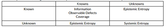
Meta-information is very useful to at least gauge the size of what we do not know, even though we do not have the information. This is essentially what the discipline of meta-mathematics was developed to do: establish, through the analysis of mathematical frameworks, what is provable and what is not provable. Even though a large proportion of mathematical propositions, like the Continuum Hypothesis regarding the existence of certain infinite cardinals, cannot be proven, it doesn’t cause problems for the mathematical community since it is possible to focus on propositions that can be proved. The same should apply to testing: using analogous methods it is possible to concentrate on those things that can be tested (i.e. the known knowns) and settle on meta-information about the rest of them. Unknown unknowns (i.e. systemic entropy) are a problem, since these cannot be measured. But the two other sections (known unknowns and unknown knowns) can at least be measured, hence statistics can be derived, which is extremely useful for risk analysis.
The core idea of this analogy, which I tentatively call “meta-development”, is the idea that testable software (i.e. known knowns) should be focused on, and all efforts should be directed at maximizing the information that is available and observable – meta-information is sufficient for the rest. Current test case design methodologies sadly do not make the most of the available information, as will be considered in our critique. Although it is true that “most” algorithms, in terms of Turing machines, are untestable (as by the Halting Problem showed), there is still an infinite number of configurations that can be tested, at least up to 100% functional coverage. In this context, I use the measure- theoretic concept of relative size to compare infinite sets – the set of untestable algorithms forms the majority of the total number of algorithms (i.e. an uncountably infinite number), whereas the set of testable algorithms form a negligible subset (a countably infinite number, which in measure theory is considered a “set of measure 0” or a “null set”, which are effectively infinitesimally small by comparison).
A Critique of Test Case Design – Methods
Given the fundamental tenets above, we now move towards providing an objective critique of test case design methods. Bearing in mind the first tenet, it will not be possible to uncover all defects. However, given the second, third and fourth tenets, we have criteria by which we rate test case design methods:
- How much application information can be encoded into the test case design process?
- How many defects are made observable?
- Coverage: how many defects are made observable by this method as a proportion of the theoretical maximum number of observable defects?
- Relative number of test cases required to reach optimum coverage.
Based on these four criteria, each test case design method will be given a score out of 10, assessing its:
- Capability of encoding – this is the amount of quantitative information about the application that can be encoded
into the method. (Derived from Number 1, above).
- Ease of encoding – how easy it is to encode the information.
- Applicability – how many scenarios can be sensibly encoded using the method.
- # of test cases – the relative number of test cases generated (1 – too few/too many, 10 – optimal). (Number 4,
above).
- Detectable Defects – the relative number of defects that can be found. (Derived from Number 2, above).
- Coverage – the relative functional coverage that can be attained. (Derived from Number 3, above).
Observable Defects in Logic
Before moving on in earnest, it is first necessary to establish a few properties of observable defects in relation to logical statements. Most formal models of testing which use application information are fundamentally dependent on the analysis of logical statements, hence it is a good place to start looking for defects.
Let us consider a very simple sentence: IF A AND B THEN C
This can be split into causes (A and B) and effects (C). In terms of defects, both of the causes can have three states: implemented correctly (OK), stuck at 0 (0) and stuck at 1 (1). But what happens when we consider the defects associated with C, given this information?
All possible defects associated with C are coded in the below table (all of the defects are highlighted in red):
| A | B | C | 1 | 1 | OK | OK | 1 1 | 0 | 0 A |
| OK | OK | 0 | 1 | 1 0 | 1 | 0 B | |||
| 0 | 0 | 1 | 1 | 1 | 1 | 1 | 1 1 | 1 | 0 |
| 0 | 1 | 1 | 0 | 1 | 1 | 1 | 1 1 | 1 | 0 |
| 1 | 0 | 1 | 1 | 1 | 0 | 1 | 1 1 | 1 | 0 |
| 1 | 1 | 0 | 0 | 1 | 0 | 1 | 1 1 | 1 | 1 |
As you can see, the last three functional variations (i.e. set of true/false inputs) are sufficient to discover all possible defects – the first variation simply does not detect any further defects. Thus, it is possible to prove that all possible defects can be discovered by this methodology – this table gives the general figures for a logical operator with n inputs:
| Number of Inputs2 | Number of required functional variations3 | Number of possible combinations4 | Number of possible defects8 |
| 3 | 4 | 8 | 26 |
| 4 | 5 | 16 | 80 |
| 56 | 67 | 3264 | 242728 |
| n | n + 1 | 2 n | ∑n (n ) 2x = 3n – 1x=1 x |
As stated above, there are two classes of defects: observable and unobservable. The distinguishing factor is not that their effects are unobservable, but that their root causes are unobservable. This is absolutely critical in order to make sure we get the right answer for the right reason. Observability in this context can be thought of as the minimum information required to identify, reproduce or fix the defect – in other words, given a defect, it should be possible to pinpoint exactly where the defect has occurred. In many respects, good test case design aims to do this in reverse: provide the minimum number of test cases to expose the most observable defects. Remember, in our world, observable defects represent the epistemic entropy of the software and can be nullified and measured, whereas unobservable defects are systemic, and cannot be tested using the same model. Test coverage, therefore, is a measure of the amount of epistemic entropy that can be nullified by the testing process.
Quick and Dirty- Combinatorial Methods (All Pairs etc.)
Derived from simple counting arguments, combinatorial methods are the simplest form of test case design – simply put, given a list of columns and possible values for each, all possible combinations of pairs, triples etc. are derived and quickly populated. The most attractive property these methods have is that they do not rely on any application knowledge whatsoever; however, this is also their most fatal weakness. Hence, their quantitative information input is restricted to data, without any input as to their relationships. Following the fundamental tenet above, the qualitative information about the system revealed by such testing will also be relatively low. Since they do not map onto actual functional points whatsoever, no determination can be made as to how much of the application logic is actually being tested. In most scenarios, endemic under-testing is performed, though there are some aspects which get needlessly over-tested, due to redundant logical conditions.
Combinatorial methods have a second weakness, which is a corollary to the above: invalid data combinations are often produced, leading to false positives where it is the data that causes a test to fail and not an actual defect. This can be mitigated somewhat by introducing constraints: this goes to show that, when more quantitative input is provided, the qualitative data produced is much clearer. Thirdly, expected results cannot be factored in automatically – these, again, rely on quantitative input. Superior methods allow for the encoding for such information, thus our analysis shows that combinatorial methods are a very poor choice of test case design.
Thus, the use of combinatorial methods should be restricted to non-functional and configuration testing only: in
|
|||||||||||||||||||
other words, scenarios where the only expected result is “it works”. Scores, out of 10, for Combinatorial Methods:
Over-Specialized: Multiplicative Coverage
A highly-specialized adaptation of combinatorial methods, this method is only useful where the scenario under test is solely dependent on the number of instances of a particular data entity. For example, suppose we have a customer accounts database, and there is a screen to display all accounts for a given customer. The scenarios under test would be:
- Customer has no accounts
- Customer has a single account
- Customer has multiple accounts
Note that this technique implicitly assumes some functional logic, hence there is some application information being input into the test case design, unlike its simpler cousins. In fact, I use this technique every time I handle parent-child relations inside a relational database or hierarchical structures (such as XML). More generally, this technique finds great use when testing aggregation methods over complex data structures. This is due to the fact that some aggregation functions have special (or degenerate) cases which must be handled separately. For example:
- Taking an average of a set of numbers requires special handling for the case of an empty set – otherwise one
gets a divide-by-zero bug.
- Taking the standard deviation of a set of numbers requires special handling for both the empty set and a single- valued set – the former will lead to a negative result, and the latter a divide-by-zero, if they are not handled separately.
The qualitative output of such a method is confirmation that all possible sets of inputs work, given their size only. This is a special case of equivalence class testing, where the range of input is grouped together into disjoint classes in order to reduce the total number of test scenarios, while maintaining integrity of functional coverage.
Scores, out of 10, for Multiplicative Coverage Methods:
| Input Information | Output Information | ||||
| Capability | Ease | Appicability | # of Test Cases | Detectable Defects | Coverage |
| 3 | 7 | 1 | 5 | 3 | 3 |
Formal Models – an introduction
The remainder of this article will be devoted to formal modelling techniques, which provides the most precise qualitative information about the system. As the tenet above states, this requires the most expertise since a great deal of quantitative information is required to get the most out of it. These methods are unique in terms of the amount of information that can be encoded into the test case design process.
Before we proceed, a brief description of what is meant by formal models is in order. Essentially, formal models are mathematically- precise descriptions of a requirement, where further operations can be performed that give us qualitative information about it. The most important three operations are:
- Consistency-checking: ensures that the logic of the requirement is internally consistent. This eliminates ambiguities due to contradictions.
- Completeness-checking: ensures that the logic of the requirement is complete. Thus eliminates ambiguities due to omissions.
- Derivation of expected results: consistent and complete logic will give expected results for any possible scenario, which allows test cases to have expected results derived automatically. This is the greatest strength of formal models in the eyes of a tester.
The formalisms themselves yield themselves to be more “useful”, simply by virtue of the above three operations – all of the above provide incredibly detailed qualitative information about the system under test. In fact, if introduced sooner into the development lifecycle, qualitative information can be extracted from the requirements themselves, ensuring that the project starts off with a strong foundation. Moreover, most requirements-specification methodologies are inert and useless outside the design phase (outside manual intervention), whereas formal models can provide information to all stages of the development lifecycle. Without going into too much detail, such formalisms form the bedrock on which most of the mathematical and computational progress in the last century or so have been achieved. If it is good enough for them, then it stands to reason that it is good enough for us.
Formal models come in all shapes and sizes, so I shall focus on the two that are most pertinent to testing: namely, flowcharting and cause and effect graphing. These can be thought of as the canonical forms – every formal model is somewhat similar to one of these two.
Visualizing Requirements and Systems – Flowcharts
Flowcharting, by and large, is a widely-understood form of requirements specification; its advantages over “wall of text” approaches are many, but none are more useful than the ability to derive test cases systematically from the requirements (which automated algorithms can achieve). This is more straightforward than it seems at first glance, and it is a mindset I have found to be challenging to convey.
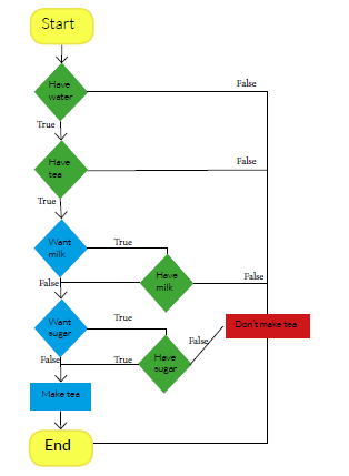
To derive test cases, one simply evaluates the possible paths through the flowchart. That, essentially, is all there is to it (formally, it is called graph homotopy analysis). Where it gets clever is when optimization techniques are applied to reduce the number of test cases, but retains functional coverage by virtue of the logical structure. In essence, one block (or operator) is fully tested considering all direct ways in and out, then the entire flow is considered fully tested. This, more than anything is extremely difficult (and frustrating) to communicate, short of exclaiming “the math works!”.
In short, it works because some paths are made redundant due to the same set of local conditions (i.e. at operator level) being tested, which happens if we try and factor other (far away, i.e. global) being tested – it is a simple fact of redundant functional variations “cancelling” each other out. It is one of those things that is easier to explain in general than it is for specific instances (as it is for much of abstract mathematics).
Since flowcharts allow for unambiguous requirements to be specified, the amount of quantitative information that is able to be encoded is huge – several orders of magnitude greater than the two previous methods. This is, again, true of all formal modelling methods – the only differences are in the degree. In addition, due to the concept of operator-level testing, the amount of defects that can be detected is also very large, hence the amount of qualitative information obtained from the model is correspondingly very large.
Scores, out of 10, for Flowcharting:
| Input Information | Output Information | ||||
| Capability | Ease | Appicability | # of Test Cases | Detectable Defects | Coverage |
| 9 | 9 | 9 | 9 | 9 | 9 |
Since flowcharts allow for unambiguous requirements to be specified, the amount of quantitative information that is able to be encoded is huge – several orders of magnitude greater than the two previous methods.
Hardcore Logic Specification – Cause and Effect Graphs
Another example of a formal model – this time, logical statements are modelled as causes and effects, and the relationship between them are fully specified. Like flowcharts, this one has been specifically analyzed due to its capability of ensuring that prose requirements are specified in an unambiguous way.
The idea is, like a flowchart, blocks are linked together, except this time it is causal relationships that are being specified. In addition, blocks are linked together using logical operators, such as AND, OR and NOT. For example, the sentence “if A or B then C” can be encoded as follows:

It should be apparent that information can be encoded in an extremely granular way this way, and it is considered to be among the best in this regard. However, is should also be equally apparent that the method is not at all easy, hence it is considered one of the most difficult.
However, the ability to find defects is staggering, more so than flowcharting, since defects can be analytically derived from a logical condition – see the section on “observable defects from logic” for an in-depth explanation of the process. In particular, it is possible to prove that all possible defects can be discovered by this methodology. As a result, this methodology is by far the best in terms of discovering observable defects, though it is very difficult compared to flowcharting, which has unfortunately stymied its adoption. In particular, its difficulty lies in attempting to encode order-specific requirements (as opposed to flowcharts which are ideal for this purpose, though they suffer from not being able to encode order-independent requirements well).
Scores, out of 10, for Cause and Effect Graphs:
| Input Information | Output Information | ||||
| Capability | Ease | Appicability | # of Test Cases | Detectable Defects | Coverage |
| 10 | 5 | 8 | 10 | 10 | 10 |
Relative Comparison
The below table is a comparison of the general scores of all the test case design methods shown above – all scores are between 1 and 10 and, while being as objective as possible, are judged according to the following criteria discussed above:
- Capability of encoding – this is the amount of quantitative information about the application that can be encoded into the method.
- Ease of encoding – how easy it is to encode the information.
- Applicability – how many scenarios can be sensibly encoded using the method.
- # of test cases – the relative number of test cases generated (1 – too few/too many, 10 – optimal).
- Detectable Defects – the relative number of defects that can be found.
- Coverage – the relative functional coverage that can be attained.
NOTE: Included also are the class of formal models which are included in one category – the scores are included as a range, as some are more capable, less applicable etc. than others.
| Method | Input Information | Output Information | ||||
| Capability | Ease | Applicability | # of Test Cases | DetectableDefects | Coverage | |
| Combinatoric | 1 | 9 | 5 | 2 | 1 | 1 |
| Multiplicative | 3 | 7 | 1 | 5 | 3 | 3 |
| Formal Models(general) | 7-10 | 5-10 | 5-10 | 5-10 | 5-10 | 5-10 |
| Flowcharting | 9 | 9 | 9 | 9 | 9 | 9 |
| Cause andEffect | 10 | 5 | 8 | 10 | 10 | 10 |
If you have any questions, or would like to talk through any ideas discussed in this paper then please contact Llyr: llyr.jones@grid-tools.com.